Quanser Aero PID Control Design
AE 443 · Experimental Dynamics & Control Laboratory · Spring 2026 · ERAU
Role
Team Member — PID Tuning & System Identification
AE 443: Experimental Dynamics & Control · ERAU · Spring 2026
Tools
MATLAB · Simulink · QUARC Real-Time Control
Transfer Function Analysis · Bode / Frequency Response
Key Contributions
- Tuned PID controller (kp = 8, kd = 3.1, ki = 5) achieving 4.12% overshoot against a sub-16.7% design spec
- Identified second-order plant model from experimental step response: ζ = 0.0452, ωn = 2.18 rad/s
- Derived analytical PID gains from pole-placement and verified phase margin improvement from 3.68° to 87.5°
- Compared model-based and manually tuned controllers, demonstrating why empirical tuning outperformed the analytical design for tracking a square-wave command
This page walks through the pitch-axis control design for the Quanser Aero lab platform — from characterizing the open-loop dynamics, through individually tuning each PID term, to deriving an analytical second-order model and comparing it against the empirically tuned controller.
System Description & Objectives
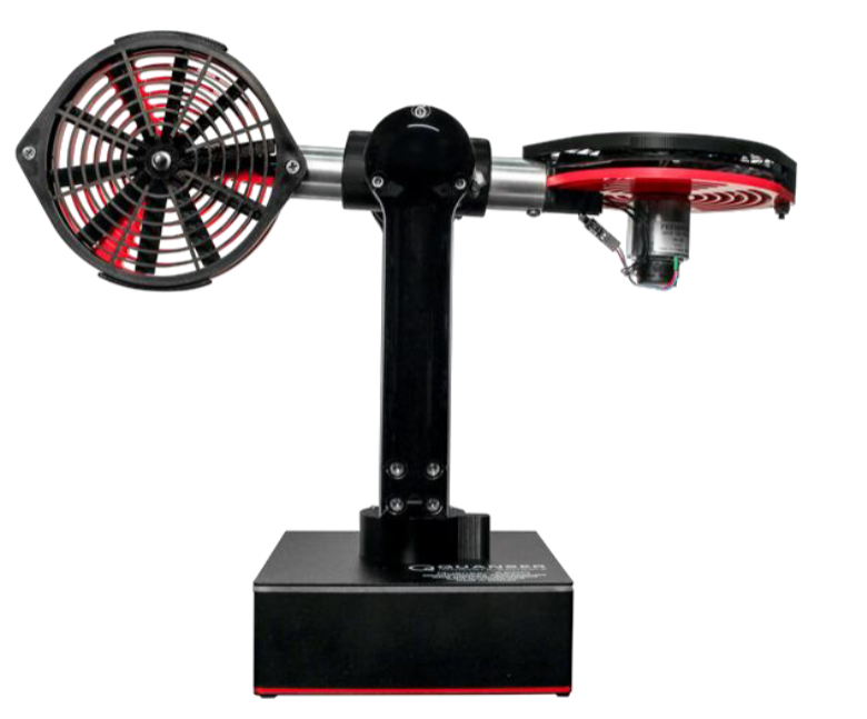
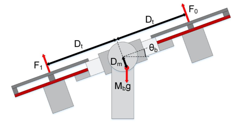
The Quanser Aero is a two-degree-of-freedom laboratory platform that mimics the pitch and yaw dynamics of a helicopter body. Two brushless DC motors drive propellers mounted at the ends of a rigid arm; the resulting thrust forces create moments about the pitch axis (elevation) and the yaw axis (travel). The platform is instrumented with encoders on both axes and connects to a host PC through QUARC real-time software, which closes the control loop in hardware at millisecond sampling rates. Because the aerodynamic coupling, inertia, and motor dynamics are all present, the Quanser Aero provides a physically meaningful testbed for classic control techniques well beyond pure simulation.
This project focused exclusively on the pitch axis. The objectives were:
- Characterize the open-loop pitch response and extract key transient parameters (ωn, ζ, settling time)
- Systematically study the individual effects of proportional, derivative, and integral control action on response speed, damping, and steady-state error
- Tune a PID controller to meet design requirements: peak pitch ≤ 0.35 rad and peak time < 1.1 s for a 0.3 rad square-wave command
- Develop a second-order plant model from experimental data and use it to calculate PID gains analytically, then compare with the tuned controller
- Evaluate closed-loop stability margins using Bode analysis in MATLAB
Open-Loop System Characterization
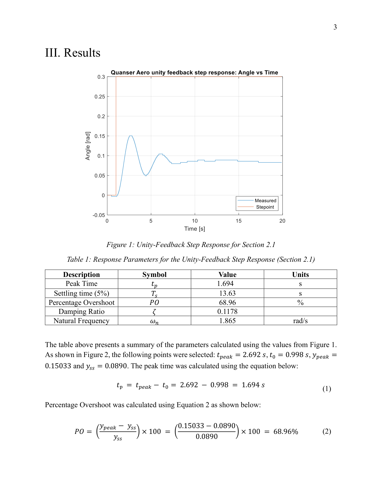
The experiment began with a unity-feedback step response on the uncompensated pitch axis to measure baseline dynamics. From the measured response, the following key points were identified:
- tpeak = 2.692 s · t0 = 0.998 s (step onset) · ypeak = 0.15033 rad · yss = 0.0890 rad
These values were used to compute the standard second-order metrics:
| Parameter | Symbol | Value |
|---|---|---|
| Peak Time | tp | 1.694 s |
| Settling Time (5%) | Ts | 13.63 s |
| Percentage Overshoot | PO | 68.96% |
| Damping Ratio | ζ | 0.1178 |
| Natural Frequency | ωn | 1.865 rad/s |
With a damping ratio of ζ = 0.1178, the uncompensated Quanser Aero pitch axis is highly underdamped. The 68.96% overshoot and 13.63-second settling time confirm that compensation is required before the platform can track any meaningful command.
Effect of Each Control Action on Pitch Response
Proportional Gain
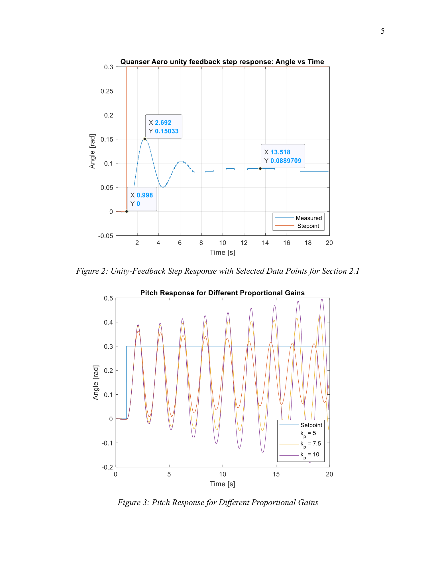
Proportional gain kp was varied from 5 to 10 in steps of 2.5.
- Increasing kp decreased peak time only slightly — from ~1.17 s at kp = 5 to ~1.1 s at kp = 10
- Percentage overshoot grew sharply, from ~20% up past 60%, with oscillations that failed to decay at the highest gain
Proportional control alone could not satisfy both the peak time and overshoot requirements simultaneously.
Derivative Gain
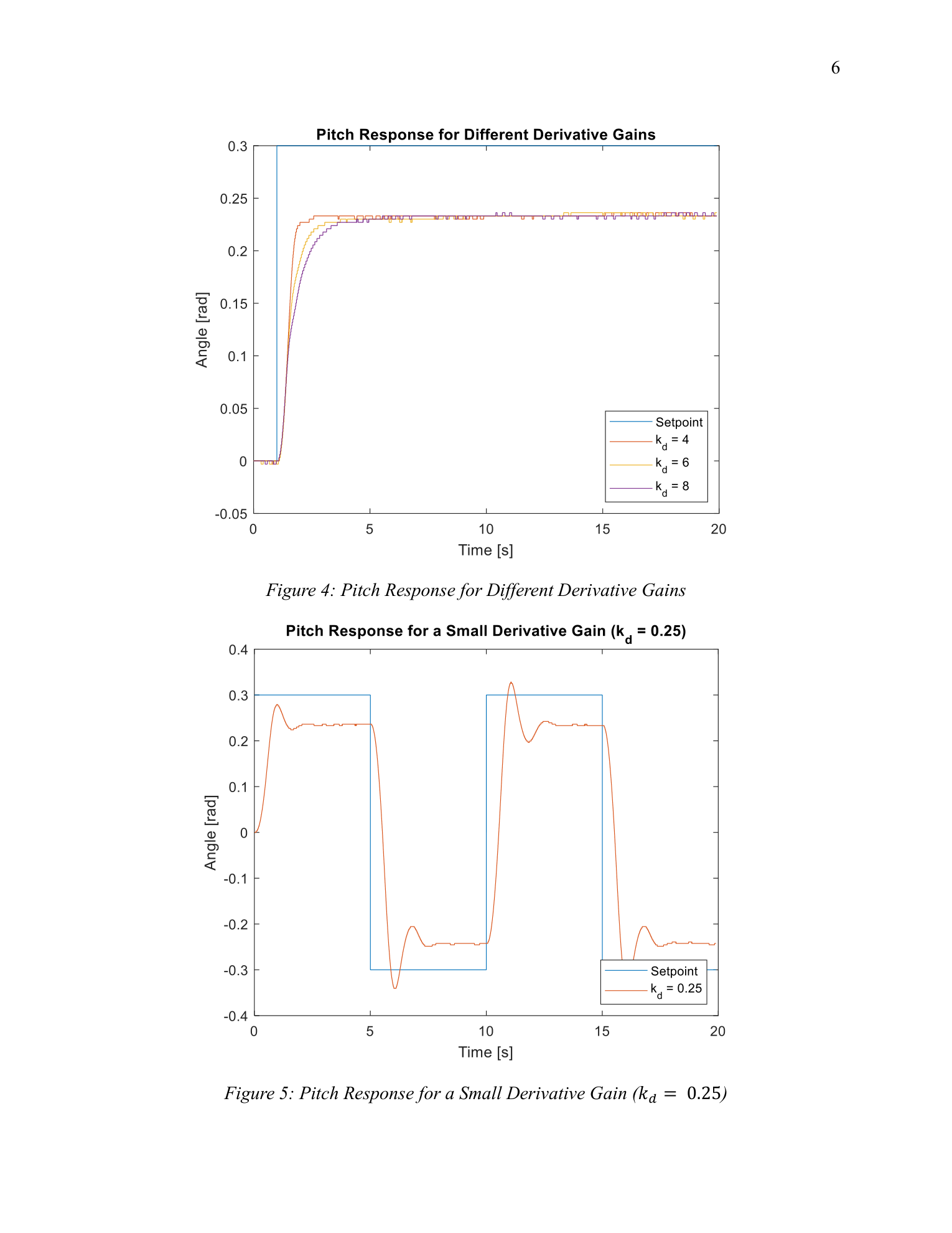
Derivative gain kd was varied from 4 to 8 in steps of 2, with kp held fixed.
- All three values produced zero percent overshoot — a significant improvement
- The tradeoff was increasing peak time, from ~1.6 s at kd = 4 to ~2.6 s at kd = 8
- A secondary test at kd = 0.25 showed the expected fast but oscillatory response, confirming the damping role of the derivative term
Integral Gain
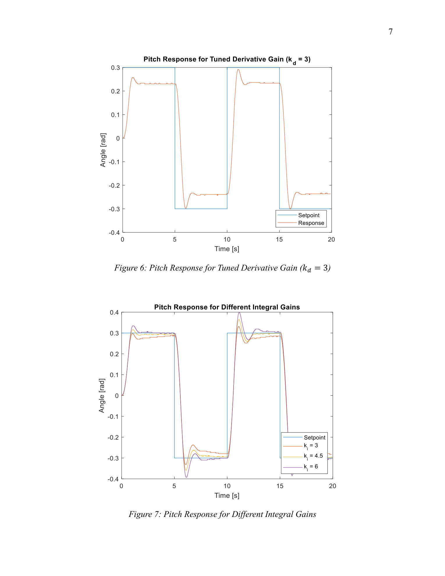
With the square-wave input active, integral gain ki was varied from 3 to 6 in steps of 1.5.
- At ki = 3, the system tracked below the setpoint
- At ki = 6, steady-state error was nearly eliminated, but overshoot grew to ~0.4 rad and inter-cycle oscillations became pronounced
- A tuned value of ki = 5 gave a steady-state pitch of 0.2976 rad (setpoint: 0.3 rad) with controlled overshoot
Final PID Tuning & Performance
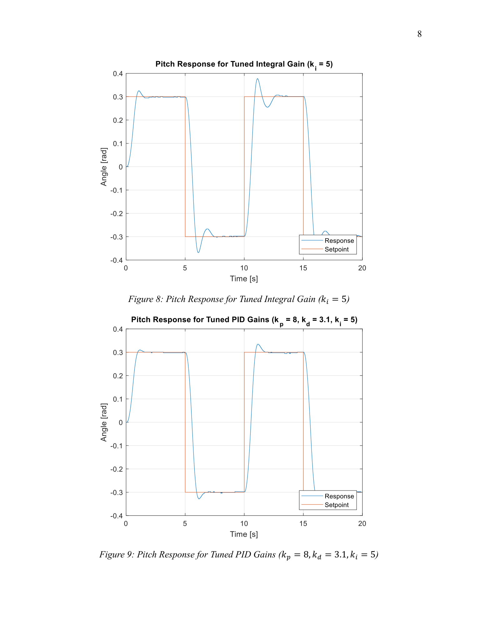
The three gains were tuned simultaneously on the hardware until the combined response met all design requirements. The final tuned gains were kp = 8, kd = 3.1, ki = 5. These values were chosen by first setting kp high enough for fast rise, then adding kd to suppress oscillations, and finally increasing ki incrementally to drive out the remaining steady-state error without reintroducing instability.
| Parameter | Value | Specification | Met? |
|---|---|---|---|
| Peak Time (tp) | 1.18 s | < 1.1 s | ✗ (marginal) |
| Percentage Overshoot | 4.12% | Peak ≤ 0.35 rad | ✓ |
| Steady-State Value | 0.2976 rad | ~0.3 rad | ✓ |
Second-Order System Identification & Analytical PID Design
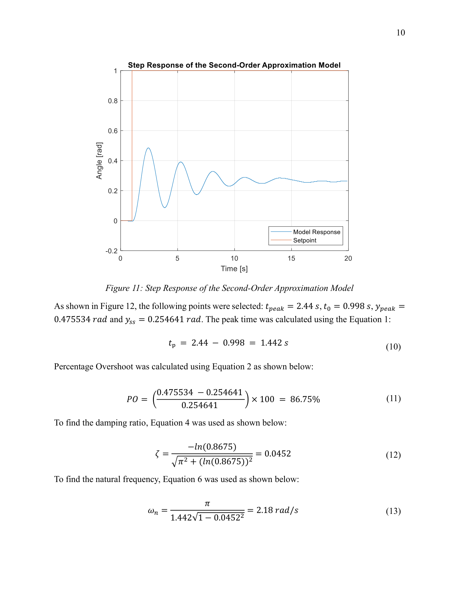
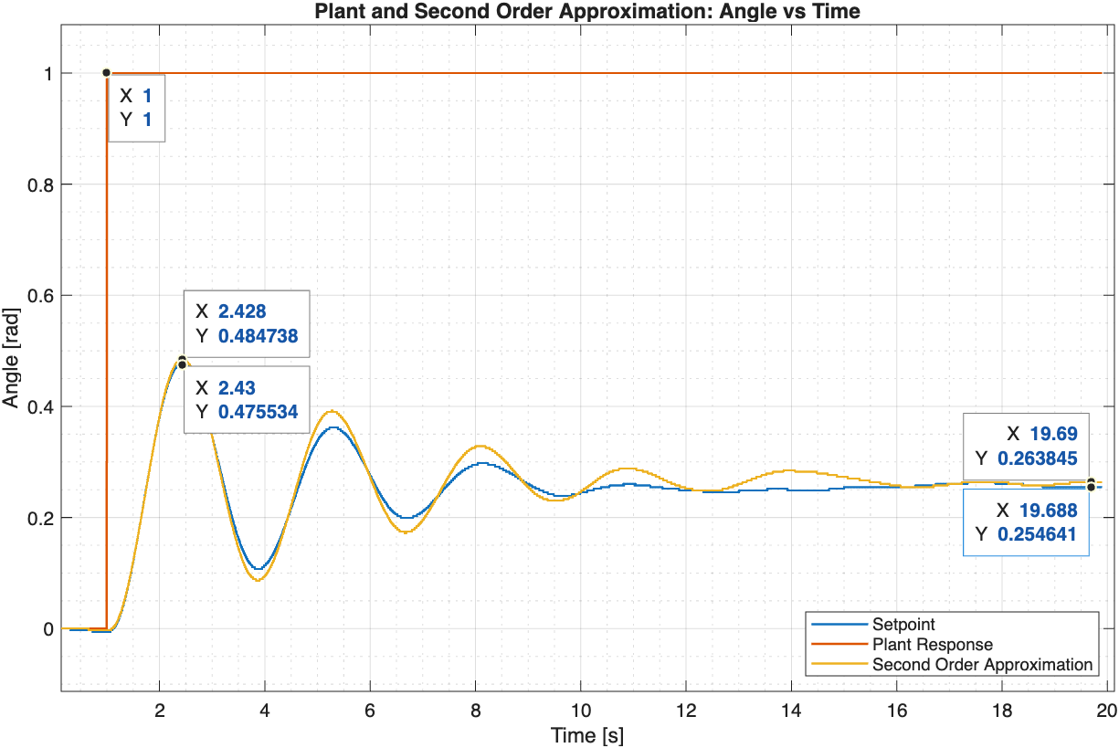
A second independent step response was recorded under unity feedback to derive a second-order plant model. From the measured data (ypeak = 0.4755 rad, yss = 0.2546 rad, tp = 1.442 s), the following model parameters were calculated:
- Percentage Overshoot: 86.75%
- Damping Ratio: ζ = 0.0452
- Natural Frequency: ωn = 2.18 rad/s
The resulting second-order transfer function approximating the Quanser Aero pitch axis is:
G(s) = 1.27332 / (s2 + 0.10047s + 3.62403)
To validate the model, its simulated step response was overlaid with the experimental plant response. The agreement was strong: peak time error was only 0.14%, percent overshoot error was 3.48%, and steady-state difference was 3.61%. The small errors confirm the approximation captures the dominant dynamics well, though higher-order effects (friction, actuator saturation) prevent a perfect match.
Analytically Calculated PID Gains
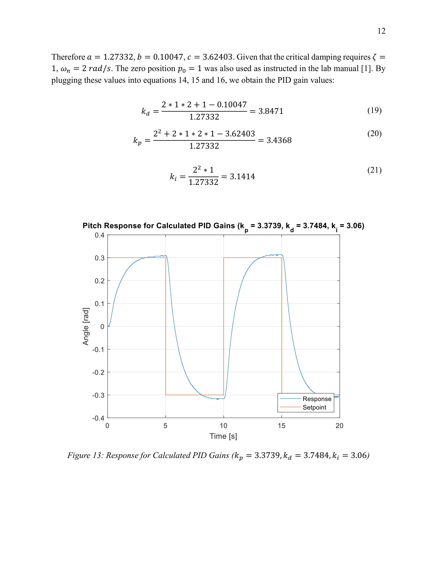
Using the identified transfer function coefficients (a = 1.27332, b = 0.10047, c = 3.62403) and a target of critically damped response (ζd = 1, ωnd = 2 rad/s) with integrator zero p0 = 1, the three PID gains were solved analytically:
- kd = (2ζdωnd + p0 − b) / a = 3.847
- kp = (ωnd2 + 2ζdωndp0 − c) / a = 3.437
- ki = ωnd2p0 / a = 3.141
For hardware testing, the workbook solution values (kp = 3.3739, kd = 3.7484, ki = 3.06) were used. These produced a critically damped square-wave response with 0% overshoot and a peak time of 4.64 s — considerably slower than the tuned controller due to the conservative critical damping target and the limitations of the second-order approximation.
Design Decision
Trade-off: The analytically derived gains targeted a critically damped response, producing 0% overshoot but a peak time of 4.64 s — nearly four times slower than the empirically tuned controller's 1.18 s.
Why: The conservative critical-damping target, combined with the second-order model's limitations (it does not capture friction or actuator saturation), made the analytical gains too sluggish for square-wave tracking. Empirical tuning of kp = 8, kd = 3.1, ki = 5 on the actual hardware compensated for these unmodeled effects and met the speed requirement directly.
Frequency-Domain Analysis & Stability Margins
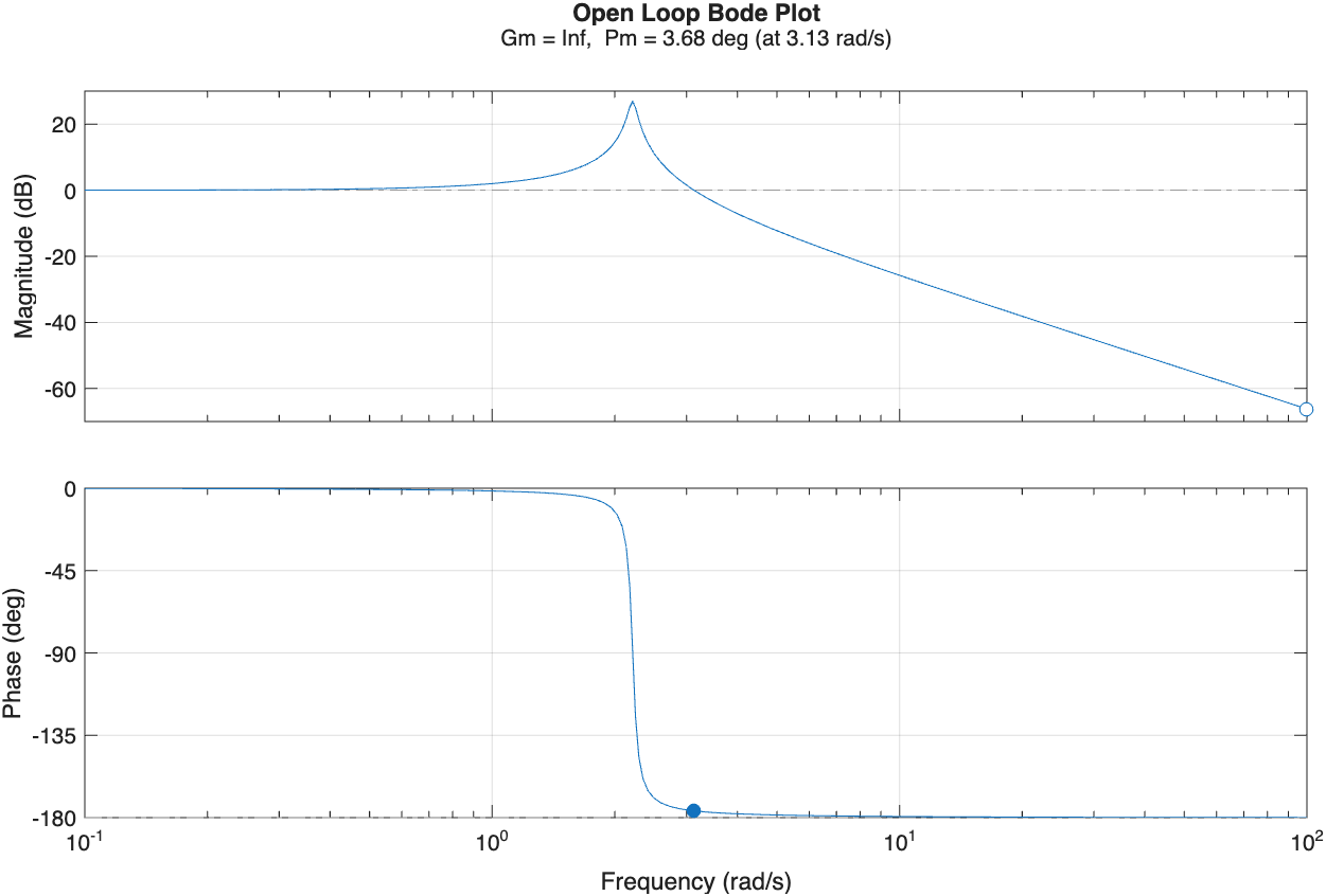
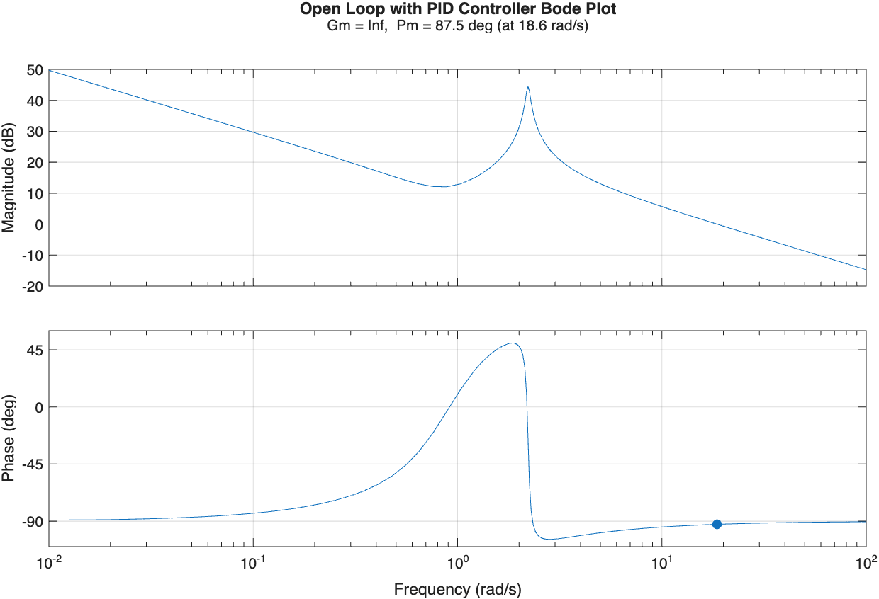
Bode plots were generated in MATLAB for both the open-loop plant and the PID-compensated open loop. The plant transfer function G(s) = ωn2 / (s2 + 2ζωns + ωn2) was combined with the PID controller C(s) = kp + ki/s + kds, and the margin() function was used to extract gain margins, phase margins, and bandwidth.
| System | Phase Margin | Gain Margin | Bandwidth |
|---|---|---|---|
| Open Loop (plant only) | 3.68° | ∞ | N/A |
| PID Compensated | 87.5° | ∞ | 19.32 rad/s |
The open-loop plant has a phase margin of only 3.68°, placing it right at the edge of instability — consistent with the severe oscillations seen in the open-loop step response. Adding the PID controller drives the phase margin to 87.5°, a dramatic improvement indicating robust stability with ample damping. The gain margin is infinite for both cases because the phase never crosses −180° in the frequency range of interest.
State-Space Formulation & System Properties
The identified second-order transfer function was converted to state-space form by defining states x1 = y (pitch angle) and x2 = ˙y (pitch rate). The resulting matrices are:
A = [[0, 1], [−ωn2, −2ζωn]] B = [[0], [ωn2]] C = [1, 0] D = [0]
The controllability matrix Pc has determinant −ωn4 ≠ 0 and rank 2, confirming the system is fully controllable. The observability matrix Po = I2×2, so det(Po) = 1 and rank = 2, confirming full observability. Although the system satisfies the necessary conditions for state-feedback control, PID remains the more practical choice here: the plant is simple enough that the additional complexity of a full state observer is not justified.
Key Takeaways
Manual tuning outperformed model-based design for tracking a square-wave command.
The analytically calculated gains produced 0% overshoot but tracked the command too slowly (tp = 4.64 s vs. 1.18 s for the tuned controller). The second-order model was adequate for linear analysis but missed friction, actuator limits, and higher-order dynamics that empirical tuning naturally compensated for.
PID compensation transformed a nearly unstable plant into a robustly stable closed loop.
The open-loop Quanser Aero pitch axis had a phase margin of only 3.68° — one small perturbation from instability. Adding the PID controller raised the phase margin to 87.5°, transforming a poorly damped (ζ = 0.0452) system into one with reliable, repeatable square-wave tracking.
Each gain has a distinct, quantifiable trade-off between speed and stability.
Increasing kp alone pushed overshoot past 60%; increasing kd alone pushed peak time past 2.6 s; increasing ki alone caused oscillations at the square-wave transitions. The final tuned combination (kp = 8, kd = 3.1, ki = 5) balanced all three effects to satisfy both speed and damping requirements simultaneously.
A second-order step-response model can capture dominant dynamics with <4% error.
The identified transfer function G(s) = 1.27332 / (s2 + 0.10047s + 3.62403) reproduced the hardware step response with 0.14% peak-time error and 3.48% overshoot error. This validates the second-order approximation method as a fast, practical tool for controller pre-design, even when the real plant contains unmodeled nonlinearities.